Gold or Bonds? Optimal S&P 500 Hedges in Shifting Macro Regimes
Published:
This article explores how to hedge the S&P 500 using gold and US Treasuries across different economic regimes.
Asset allocators frequently seek to protect equity portfolios from the impact of adverse macroeconomic shifts. Equity market drawdowns are common during periods of elevated inflation or weak economic growth. But the optimal hedge often depends on the specific macro regime. This analysis addresses a portfolio management question: Which asset provides the most effective hedge for US equities under different economic conditions?
Macroeconomic environments are classified into distinct regimes using combinations of inflation and GDP growth trends, measured on a year by year basis. For each regime, the effectiveness of gold and US Treasuries as hedges for the S&P 500 is evaluated to focus on risk adjusted performance during each phase.
Data for this study is drawn from a multi-sheet Excel file, structured as follows:
- Macro sheet - Includes key indicators such as CPI inflation, GDP growth, and policy rates
- Prices sheet - Contains historical data for the S&P 500, gold, and US dollar index
- Yield sheet - Provides US Treasury yields, with a focus on the 10-year benchmark
Python is used throughout for data processing, feature engineering, regime classification, and hedge evaluation. Familiarity with basic macroeconomics and portfolio construction will be helpful for readers following this workflow.
The methodology presented here is one of several possible approaches. This analysis offers a perspective on aligning equity hedges with prevailing macroeconomic conditions.
Step 1: Data Loading and Preparation
This analysis starts with 3 structured datasets covering US macroeconomic indicators, asset prices, and Treasury yields. The data is sourced from an Excel file and is prepared for analysis in Python.
1.1 Import Required Libraries
The following libraries are used for data manipulation, visualization, and regression analysis:
import pandas as pd
import numpy as np
import matplotlib.pyplot as plt
import statsmodels.api as sm
import seaborn as sns
1.2 Load and Inspect Data
excel_file = "Data_S&P500.xlsx"

# Read each sheet from the Excel file
df_macro = pd.read_excel(excel_file, sheet_name="Macro")
df_prices = pd.read_excel(excel_file, sheet_name="Prices")
df_yield = pd.read_excel(excel_file, sheet_name="Yield")

# Convert the 'Date' column to datetime format in each dataframe, just to make sure
for df in [df_macro, df_prices, df_yield]:
    df['Date'] = pd.to_datetime(df['Date'])

# Sort data by Date
df_macro.sort_values('Date', inplace=True)
df_prices.sort_values('Date', inplace=True)
df_yield.sort_values('Date', inplace=True)

# Check the first few rows
print("Macro Data Sample")
print(df_macro.head(10))
print("\nPrices Data Sample")
print(df_prices.head(10))
print("\nYield Data Sample")
print(df_yield.head(10))
Output:
Macro Data Sample
        Date  GDP YOY  CPI YOY
0 1970-12-31     -0.2      5.6
1 1971-01-31      NaN      5.3
2 1971-02-28      NaN      5.0
3 1971-03-31      2.7      4.7
4 1971-04-30      NaN      4.2
5 1971-05-31      NaN      4.4
6 1971-06-30      3.1      4.6
7 1971-07-31      NaN      4.4
8 1971-08-31      NaN      4.6
9 1971-09-30      3.0      4.1

Prices Data Sample
        Date  S&P 500   Gold  USD Index Spot Rate
0 1970-12-31    92.15  37.44              120.643
1 1971-01-04    91.15    NaN              120.530
2 1971-01-05    91.80    NaN              120.520
3 1971-01-06    92.35    NaN              120.490
4 1971-01-07    92.38    NaN              120.550
5 1971-01-08    92.19    NaN              120.530
6 1971-01-11    91.98    NaN              120.530
7 1971-01-12    92.72    NaN              120.490
8 1971-01-13    92.56    NaN              120.470
9 1971-01-14    92.80    NaN              120.440

Yield Data Sample
        Date  US 10YR Bonds
0 1970-12-31          6.502
1 1971-01-04          6.462
2 1971-01-05          6.472
3 1971-01-06          6.472
4 1971-01-07          6.452
5 1971-01-08          6.442
6 1971-01-11          6.392
7 1971-01-12          6.352
8 1971-01-13          6.292
9 1971-01-14          6.222
The Excel file provides 3 key datasets. The Macro sheet covers about 600 monthly observations, tracking indicators like CPI inflation, GDP growth, and policy rates. The Prices sheet holds roughly 14,000 daily records for the S&P 500, gold, and the US dollar index. The Yield sheet includes a similar number of daily entries for US 10-year Treasury yields.
Step 2: Asset Return Construction
To enable regime based analysis, monthly returns are computed for equities (S&P 500), gold, and US Treasuries. Each asset class requires a different methodology reflecting its characteristics.
2.1 Calculate S&P 500 and Gold Returns
Returns for the S&P 500 and gold are calculated as simple percentage changes in price.
# Compute percentage change returns for the S&P 500 and Gold
df_prices['SP500_ret'] = df_prices['S&P 500'].pct_change()
df_prices['Gold_ret']  = df_prices['Gold'].pct_change()
2.2 Estimate Treasury Returns via Modified Duration
Returns for US Treasuries are estimated using a duration based approach that accounts for interest rate sensitivity. For each month, the bond return is approximated as the negative of the modified duration multiplied by the change in yield:
Bond Return ≈ –(Modified Duration) × (ΔYield)
The modified duration is computed for a hypothetical 10-year par bond with the coupon rate set equal to the prevailing yield in each period.
def compute_modified_duration(y, coupon, maturity=10, par=100):
    """
    Calculate the modified duration of an annual coupon bond given the yield, coupon rate, maturity & par value

    Parameters:
      y (float): yield per period in decimal form
      coupon (float): annual coupon rate in decimal form
      maturity (int): maturity of the bond in years
      par (float): par value of the bond

    Returns:
      float: modified duration
    """
    # Generate the cash flowss
    # For years 1 to maturity-1, the cash flow is the coupon payment
    # At maturity, the cash flow includes the final coupon plus the par value
    cash_flows = [coupon * par] * (maturity - 1) + [coupon * par + par]

    # Compute discount factors for each time period
    discount_factors = [1 / (1 + y)**t for t in range(1, maturity + 1)]

    # Calculate bond price as the sum of discounted cash flows
    price = sum(cf * d for cf, d in zip(cash_flows, discount_factors))

    # Calculate Macaulay Duration as the weighted average time of cash flows
    macaulay_duration = sum(t * cf / (1 + y)**t for t, cf in zip(range(1, maturity + 1), cash_flows)) / price

    # Modified Duration adjusts Macaulay Duration by the yield
    mod_duration = macaulay_duration / (1 + y)
    return mod_duration
The 10-year Treasury yield is first converted from percent to decimal and used as both the yield and coupon for the duration calculation. Bond returns are then calculated as follows:
# Convert the US 10YR Bonds yield from percent to decimals
df_yield['Yield_decimal'] = df_yield['US 10YR Bonds'] / 100

# Determine the coupon rate from each observation
# For a par bond, coupon rate is equal to the yield
df_yield['Coupon'] = df_yield['Yield_decimal']

# Compute the modified duration for each observation using the current yield as the coupon
df_yield['Mod_Dur'] = df_yield.apply(lambda row: compute_modified_duration(row['Yield_decimal'], row['Coupon'], maturity=10), axis=1)

# Compute the change in yield ( decimal form)
df_yield['Yield_change_decimal'] = df_yield['Yield_decimal'].diff()

# Calculate the bond return using the modified duration (data-driven) and the observed yield change
df_yield['Bond_ret'] = - df_yield['Mod_Dur'] * df_yield['Yield_change_decimal']

# Display the first few rows with our computed variables
print("\nUS Treasury Data with Computed Modified Duration and Bond Returns:")
print(df_yield[['Date', 'US 10YR Bonds', 'Yield_decimal', 'Coupon', 'Mod_Dur', 'Yield_change_decimal', 'Bond_ret']].head(10))
Output:
US Treasury Data with Computed Modified Duration and Bond Returns:
        Date  US 10YR Bonds  Yield_decimal   Coupon   Mod_Dur   Yield_change_decimal  Bond_ret
0 1970-12-31          6.502        0.06502  0.06502  7.188157                    NaN       NaN
1 1971-01-04          6.462        0.06462  0.06462  7.201631                -0.0004  0.002881
2 1971-01-05          6.472        0.06472  0.06472  7.198259                 0.0001 -0.000720
3 1971-01-06          6.472        0.06472  0.06472  7.198259                 0.0000 -0.000000
4 1971-01-07          6.452        0.06452  0.06452  7.205006                -0.0002  0.001441
5 1971-01-08          6.442        0.06442  0.06442  7.208383                -0.0001  0.000721
6 1971-01-11          6.392        0.06392  0.06392  7.225304                -0.0005  0.003613
7 1971-01-12          6.352        0.06352  0.06352  7.238884                -0.0004  0.002896
8 1971-01-13          6.292        0.06292  0.06292  7.259328                -0.0006  0.004356
9 1971-01-14          6.222        0.06222  0.06222  7.283290                -0.0007  0.005098
This method provides a consistent monthly return series for US Treasuries. It also allows for direct comparison with equity and gold returns in later analysis.
Step 3: Economic Regime Classification
Economic regimes are defined by joint states of inflation and real economic growth.
3.1 Define Regimes Using Inflation and Growth
Regime construction uses median splits for both CPI YoY (as a proxy for realized inflation) and GDP YoY (for real growth). This yields a two by two grid, capturing 4 distinct macroeconomic environments. Median splits ensure equal representation across the sample and avoid arbitrary thresholding.
# Create four regimes using median splits of each indicator
cpi_median = df_macro['CPI YOY'].median()
gdp_median = df_macro['GDP YOY'].median()

# Create regime flags based on the median splits.
df_macro['Inflation_Regime'] = np.where(df_macro['CPI YOY'] >= cpi_median, 'High Inflation', 'Low Inflation')
df_macro['Growth_Regime']    = np.where(df_macro['GDP YOY'].fillna(method='ffill') >= gdp_median, 'High Growth', 'Low Growth')

# Combine the flags to create a composite regime label.
df_macro['Regime'] = df_macro['Inflation_Regime'] + " & " + df_macro['Growth_Regime']

# Review the distribution of economic regimes.
print("\nEconomic Regime Distribution:")
print(df_macro['Regime'].value_counts())
Output:
Economic Regime Distribution:
Regime
High Inflation & High Growth    192
Low Inflation & Low Growth      182
Low Inflation & High Growth     141
High Inflation & Low Growth     136
This regime definition process produces four macroeconomic states based on the joint distribution of realized inflation and real GDP growth relative to their historical medians. The sample is approximately balanced across regimes, with each state containing between 136 and 192 observations. This approach avoids arbitrary parameter choices and maintains robustness to outliers or structural changes. By forward filling missing growth values before classification, the method ensures each observation is assigned unambiguously. All subsequent analysis including asset return behavior and hedge effectiveness, is conducted conditional on these regime labels.
Step 4: Merging Datasets
4.1 Merge Macro, Price, and Yield Data
To align macroeconomic indicators with asset returns at a monthly frequency, the datasets are merged on the Date field. The macro data is first combined with S&P 500 and gold returns, followed by a merge with the calculated Treasury bond returns. Only dates with complete information across all sources are retained. This ensures consistent coverage for all subsequent analysis.
# Merge the macroeconomic data with asset returns on the Date field
# First merge Macro and Prices (for S&P 500 and Gold returns), after that merge with the computed Bond returns
df_merge1 = pd.merge(df_macro,
                     df_prices[['Date', 'SP500_ret', 'Gold_ret']],
                     on='Date', how='inner')
df_merged = pd.merge(df_merge1,
                     df_yield[['Date', 'Bond_ret']],
                     on='Date', how='inner')

# Remove any remaining missing observations
df_merged.dropna(inplace=True)
This process produces a unified dataset containing regime labels, macro variables, and monthly return series for each asset with no missing values.
Step 5: Exploratory Data Analysis
Exploratory analysis focuses on understanding the distribution and movement of monthly returns for equities, gold, and Treasuries, both in aggregate and conditional on macro regime.
5.1 Visualize Asset Return Time Series
The time series of monthly returns for the S&P 500, gold, and Treasury bond proxy are plotted to highlight changes in return behavior and volatility across different market environments.
# Plot time series of S&P 500, Gold, and Bond returns
plt.figure(figsize=(14, 6))
plt.plot(df_merged['Date'], df_merged['SP500_ret'], label="S&P 500 Returns", alpha=0.7)
plt.plot(df_merged['Date'], df_merged['Gold_ret'], label="Gold Returns", alpha=0.7)
plt.plot(df_merged['Date'], df_merged['Bond_ret'], label="Bond Proxy Returns", alpha=0.7)
plt.xlabel("Date")
plt.ylabel("Returns")
plt.title("Asset Returns Over Time")
plt.legend()
plt.show()
Output:
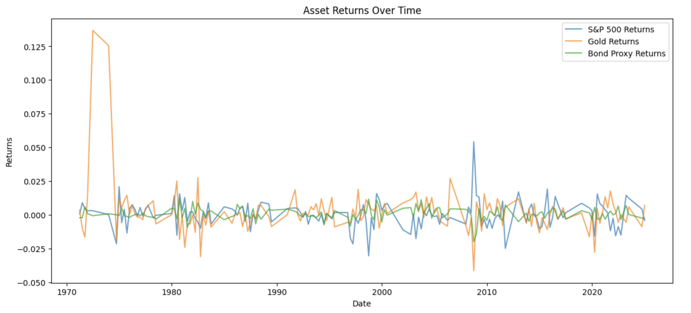
The plot of monthly returns shows equities are prone to sharp drawdowns and volatility spikes especially during crises. Gold is typically stable but has occasional outliers, most notably in the early 1970s. This reflects market regime changes. Treasury returns are consistently the least volatile. These differences emphasize that shocks rarely hit all assets at once, showing the value of analyzing hedges by regime rather than relying on long run averages.
5.2 Analyze Regime-Based Correlations
# For each economic regime, compute and plot the correlation of returns
regimes = df_merged['Regime'].unique()

for reg in regimes:
    df_reg = df_merged[df_merged['Regime'] == reg]
    corr_matrix = df_reg[['SP500_ret', 'Gold_ret', 'Bond_ret']].corr()

    print(f"\nCorrelation Matrix for {reg} regime:")
    print("----------------------------------")

    # SP500 correlations
    print(f"SP500 vs Gold: {corr_matrix.loc['SP500_ret', 'Gold_ret']:.3f}")
    print(f"SP500 vs Bonds: {corr_matrix.loc['SP500_ret', 'Bond_ret']:.3f}")

    # Gold correlations
    print(f"Gold vs Bonds: {corr_matrix.loc['Gold_ret', 'Bond_ret']:.3f}")
    print("----------------------------------")
Output:
Correlation Matrix for High Inflation & Low Growth regime:
----------------------------------
SP500 vs Gold: -0.380
SP500 vs Bonds: -0.400
Gold vs Bonds: 0.248
----------------------------------

Correlation Matrix for High Inflation & High Growth regime:
----------------------------------
SP500 vs Gold: 0.012
SP500 vs Bonds: 0.223
Gold vs Bonds: 0.139
----------------------------------

Correlation Matrix for Low Inflation & High Growth regime:
----------------------------------
SP500 vs Gold: 0.015
SP500 vs Bonds: -0.048
Gold vs Bonds: -0.059
----------------------------------

Correlation Matrix for Low Inflation & Low Growth regime:
----------------------------------
SP500 vs Gold: -0.025
SP500 vs Bonds: -0.382
Gold vs Bonds: -0.053
----------------------------------
Correlation patterns change noticeably across regimes. In stagflation, both gold and Treasuries reliably hedge the S&P 500. When growth is strong, these relationships weaken or vanish and diversification becomes harder to find. Bonds still offer some protection in slow/low-inflation periods. Gold is only a meaningful diversifier when inflation runs hot. The data makes it clear that hedge strategies need to adjust as the macro backdrop shifts.
Step 6: Optimal Hedge Ratio Estimation
6.1 Run OLS Regressions by Regime
For each economic regime, an ordinary least squares regression is run where S&P 500 returns are regressed on contemporaneous gold and bond returns. The coefficients for gold and bonds in each regression represent the conditional hedge ratios for that regime.
# Perform an OLS regression for each regime
#  1) Dependent variable: S&P 500 returns
#  2) Independent variables:Gold returns & Bond returns

# The coefficients provide the hedge ratios in each regime
results_dict = {}

for reg, group in df_merged.groupby('Regime'):
    # Prepare regression data and include an intercept term
    X = group[['Gold_ret', 'Bond_ret']]
    X = sm.add_constant(X)
    y = group['SP500_ret']

    # Fit the OLS model
    model = sm.OLS(y, X).fit()
    results_dict[reg] = model

    # Print the summary for the given regime
    print(f"==== Regression Results for {reg} ====")
    print(model.summary())
    print("\n")
Output:
==== Regression Results for High Inflation & High Growth ====
                            OLS Regression Results
==============================================================================
Dep. Variable:              SP500_ret   R-squared:                       0.050
Model:                            OLS   Adj. R-squared:                 -0.006
Method:                 Least Squares   F-statistic:                    0.8994
Date:                Sat, 12 Apr 2025   Prob (F-statistic):              0.416
Time:                        15:45:32   Log-Likelihood:                 134.63
No. Observations:                  37   AIC:                            -263.3
Df Residuals:                      34   BIC:                            -258.4
Df Model:                           2
Covariance Type:            nonrobust
==============================================================================
                 coef    std err          t      P>|t|      [0.025      0.975]
------------------------------------------------------------------------------
const          0.0005      0.001      0.422      0.676      -0.002       0.003
Gold_ret      -0.0058      0.050     -0.116      0.909      -0.108       0.097
Bond_ret       0.4063      0.303      1.339      0.189      -0.210       1.023
==============================================================================
Omnibus:                        6.015   Durbin-Watson:                   1.620
Prob(Omnibus):                  0.049   Jarque-Bera (JB):                4.795
Skew:                          -0.854   Prob(JB):                       0.0909
Kurtosis:                       3.437   Cond. No.                         278.
==============================================================================


==== Regression Results for High Inflation & Low Growth ====
                            OLS Regression Results
==============================================================================
Dep. Variable:              SP500_ret   R-squared:                       0.244
Model:                            OLS   Adj. R-squared:                  0.188
Method:                 Least Squares   F-statistic:                     4.355
Date:                Sat, 12 Apr 2025   Prob (F-statistic):             0.0229
Time:                        15:45:32   Log-Likelihood:                 88.427
No. Observations:                  30   AIC:                            -170.9
Df Residuals:                      27   BIC:                            -166.7
Df Model:                           2
Covariance Type:            nonrobust
==============================================================================
                 coef    std err          t      P>|t|      [0.025      0.975]
------------------------------------------------------------------------------
const          0.0021      0.003      0.811      0.424      -0.003       0.007
Gold_ret      -0.2893      0.167     -1.731      0.095      -0.632       0.054
Bond_ret      -0.8232      0.437     -1.886      0.070      -1.719       0.072
==============================================================================
Omnibus:                        0.183   Durbin-Watson:                   2.579
Prob(Omnibus):                  0.912   Jarque-Bera (JB):                0.334
Skew:                          -0.155   Prob(JB):                        0.846
Kurtosis:                       2.586   Cond. No.                         180.
==============================================================================


==== Regression Results for Low Inflation & High Growth ====
                            OLS Regression Results
==============================================================================
Dep. Variable:              SP500_ret   R-squared:                       0.002
Model:                            OLS   Adj. R-squared:                 -0.049
Method:                 Least Squares   F-statistic:                   0.04687
Date:                Sat, 12 Apr 2025   Prob (F-statistic):              0.954
Time:                        15:45:32   Log-Likelihood:                 143.38
No. Observations:                  42   AIC:                            -280.8
Df Residuals:                      39   BIC:                            -275.6
Df Model:                           2
Covariance Type:            nonrobust
==============================================================================
                 coef    std err          t      P>|t|      [0.025      0.975]
------------------------------------------------------------------------------
const         -0.0017      0.001     -1.219      0.230      -0.004       0.001
Gold_ret       0.0043      0.059      0.073      0.942      -0.115       0.124
Bond_ret      -0.0868      0.297     -0.292      0.772      -0.688       0.514
==============================================================================
Omnibus:                       13.967   Durbin-Watson:                   1.921
Prob(Omnibus):                  0.001   Jarque-Bera (JB):               19.470
Skew:                          -0.962   Prob(JB):                     5.92e-05
Kurtosis:                       5.724   Cond. No.                         233.
==============================================================================


==== Regression Results for Low Inflation & Low Growth ====
                            OLS Regression Results
==============================================================================
Dep. Variable:              SP500_ret   R-squared:                       0.148
Model:                            OLS   Adj. R-squared:                  0.103
Method:                 Least Squares   F-statistic:                     3.307
Date:                Sat, 12 Apr 2025   Prob (F-statistic):             0.0474
Time:                        15:45:32   Log-Likelihood:                 137.67
No. Observations:                  41   AIC:                            -269.3
Df Residuals:                      38   BIC:                            -264.2
Df Model:                           2
Covariance Type:            nonrobust
==============================================================================
                 coef    std err          t      P>|t|      [0.025      0.975]
------------------------------------------------------------------------------
const          0.0013      0.001      0.910      0.368      -0.002       0.004
Gold_ret      -0.0424      0.141     -0.300      0.766      -0.328       0.244
Bond_ret      -0.8815      0.343     -2.567      0.014      -1.577      -0.186
==============================================================================
Omnibus:                        0.935   Durbin-Watson:                   2.321
Prob(Omnibus):                  0.627   Jarque-Bera (JB):                0.964
Skew:                           0.239   Prob(JB):                        0.618
Kurtosis:                       2.420   Cond. No.                         251.
==============================================================================
The OLS regressions provide a regime specific map of hedge effectiveness. In the high inflation, high growth regime, neither gold nor Treasuries reliably offset S&P 500 risk. The bond coefficient is positive at 0.41 and statistically insignificant. Gold’s coefficient is close to zero. This indicates that neither asset offers meaningful downside protection when inflation and growth are both elevated.
In high inflation combined with low growth, both hedge betas are negative. The bond beta is -0.82 with a p-value of 0.07, while gold’s beta is -0.29 with a p-value of 0.10. This suggests that Treasuries are the more effective hedge and gold plays a secondary role. The model’s explanatory power also rises in this regime. For low inflation, Treasuries are a robust hedge only during weak growth. The bond beta is -0.88 and statistically significant, while gold again offers no material protection. When growth is strong and inflation is low, neither asset hedges equity risk.
Overall, the results show that effective hedge ratios are strongly regime dependent and static allocations are not sufficient for equity risk management.
Step 7: Hedge Relationships and Hedge Ratio Dynamics Visualization
7.1 Visualize S&P 500 vs Hedge Asset Returns by Regime
The scatter plots below show the joint distribution of S&P 500 returns against gold and bond returns, segmented by macroeconomic regime. Each subplot corresponds to one of the 4 macro regime states. Gold and bond returns are plotted on the x-axis, S&P 500 returns on the y-axis.
# Create scatter plots of S&P 500 returns vs Gold and Bond returns, segmented by regime
fig, axes = plt.subplots(2, 2, figsize=(14, 10), sharex=True, sharey=True)
regime_list = list(regimes)
for idx, reg in enumerate(regime_list):
    ax = axes[idx//2, idx%2]
    sub_df = df_merged[df_merged['Regime'] == reg]
    ax.scatter(sub_df['Gold_ret'], sub_df['SP500_ret'], color='blue', alpha=0.5, label="Gold")
    ax.scatter(sub_df['Bond_ret'], sub_df['SP500_ret'], color='green', alpha=0.5, label="Bond")
    ax.set_title(reg)
    ax.set_xlabel("Asset Returns")
    ax.set_ylabel("S&P 500 Returns")
    ax.legend()
plt.suptitle("S&P 500 vs Hedge Assets Returns by Regime")
plt.tight_layout(rect=[0, 0, 1, 0.95])
plt.show()
Output:
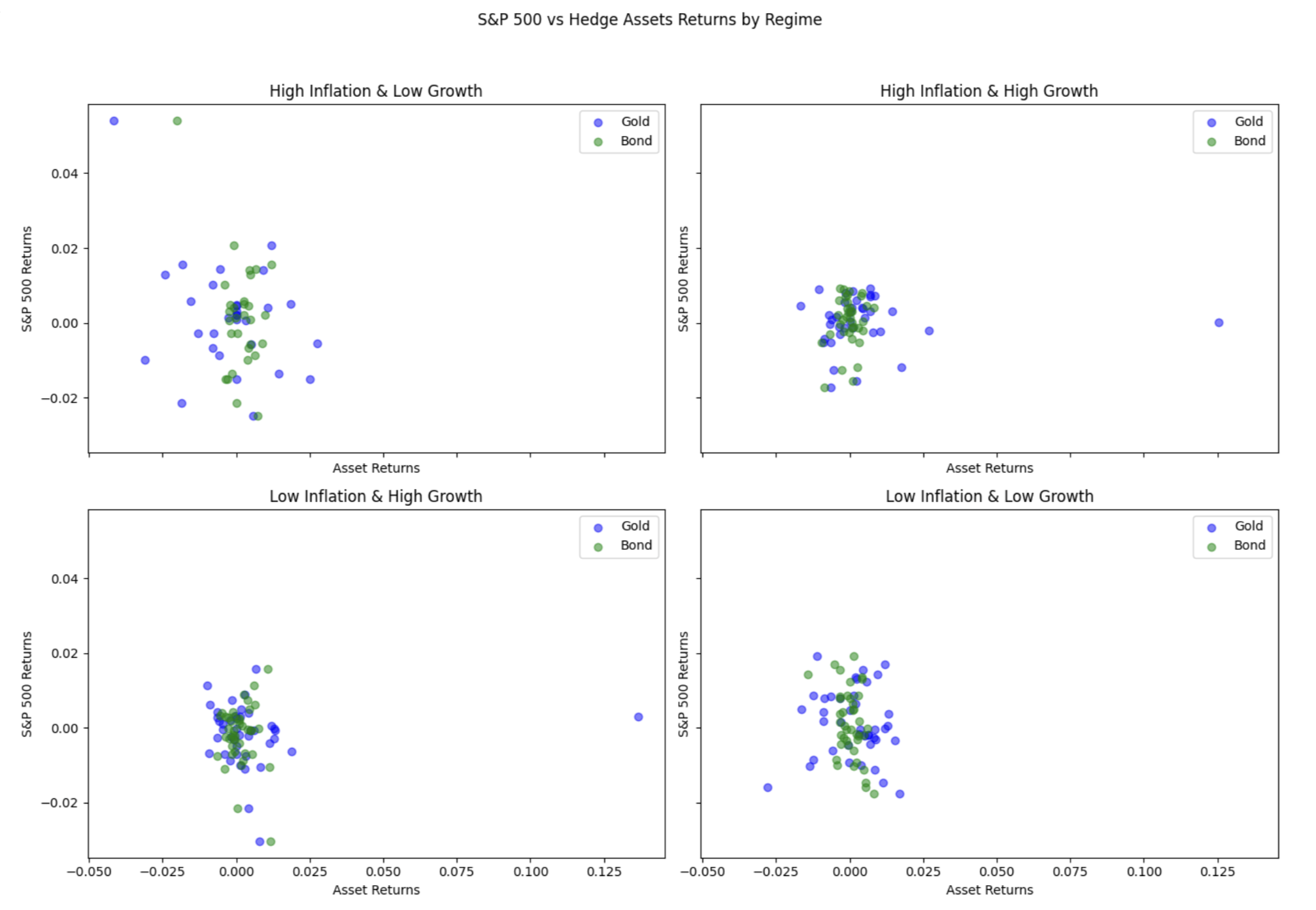
In the “High Inflation & Low Growth” regime, gold and bonds both display more pronounced negative co-movement with S&P 500 returns. This suggests greater hedging effectiveness under stagflationary stress, with more dispersion and negative slope in the scatter. In regimes with benign macro backdrops, asset return relationships are weaker and less systematic, with more clustering around the origin.
7.2 Estimate and Visualize Rolling Hedge Ratios
To capture time variation in hedge effectiveness, 36-month rolling OLS regressions are used to estimate conditional hedge ratios for gold and bonds. The resulting time series plot tracks the evolution of these coefficients.
# compute rolling regression hedge ratios using a 36 month window
window = 36
rolling_results = []

# Ensure the merged dataset is sorted by date
df_merged = df_merged.sort_values('Date').reset_index(drop=True)

for i in range(window, df_merged.shape[0]):
    window_data = df_merged.iloc[i-window:i]
    X = window_data[['Gold_ret', 'Bond_ret']]
    X = sm.add_constant(X)
    y = window_data['SP500_ret']
    model = sm.OLS(y, X).fit()
    # Record the hedge ratios (coefficients for Gold_ret and Bond_ret) along with the window's end date
    rolling_results.append({
        'Date': df_merged.loc[i, 'Date'],
        'Gold_Hedge': model.params['Gold_ret'],
        'Bond_Hedge': model.params['Bond_ret']
    })

df_rolling = pd.DataFrame(rolling_results)

# Plot the rolling hedge ratios over time
plt.figure(figsize=(12, 6))
plt.plot(df_rolling['Date'], df_rolling['Gold_Hedge'], label="Rolling Gold Hedge Ratio")
plt.plot(df_rolling['Date'], df_rolling['Bond_Hedge'], label="Rolling Bond Hedge Ratio")
plt.xlabel("Date")
plt.ylabel("Hedge Ratio")
plt.title("Rolling Hedge Ratios Over Time (36-Month Window)")
plt.legend()
plt.show()
This approach makes clear that hedge ratios are highly dynamic. Bond hedge ratios trend sharply negative during major market stress (e.g., 2008–09), with substantial protective value when equity-bond correlation turns strongly negative. Gold hedge ratios are more volatile and episodic, spiking around inflationary or geopolitical shocks but decaying in stable periods. The rolling estimation framework demonstrates that optimal hedging cannot be static and is instead sensitive to changing macro and market structure.
Step 8: Hedge Recommendations and Takeaways
8.1 Regime-Based Hedge Recommendations
| Regime | Optimal Hedge | Supporting Evidence |
|---|---|---|
| High Inflation / Low Growth | 80% Bonds, 20% Gold | Bonds: β = -0.82 (p=0.07), Gold: β = -0.29 (p=0.095). Correlations: S&P-Bonds (-0.40), S&P-Gold (-0.38). |
| Low Inflation / Low Growth | 90% Bonds | Bonds: β = -0.88 (p=0.014). Correlation: S&P-Bonds (-0.38). Rolling ratios show crisis-era stability. |
| High Inflation / High Growth | Minimal hedge | Statistically insignificant hedges. Weak correlations (S&P-Bonds: +0.22, S&P-Gold: +0.01). |
| Low Inflation / High Growth | No Hedge | Near-zero correlations and noisy regression signals. |
Hedge effectiveness is highly sensitive to the macro backdrop. During periods of high inflation coupled with weak growth (stagflation), US Treasuries provide substantial downside protection, while gold contributes a valuable, though smaller and stabilizing effect.
In low-growth, low-inflation environments, Treasuries serve as the main defensive asset due to their lower volatility and stronger inverse relation with equity returns. In robust growth scenarios, the need for hedging diminishes as correlations between risk assets weaken.
For gold, it’s only tactical in stagflation; avoid strategic allocations.
For bond, it’s critical in low-growth regimes, validated by correlations and rolling ratios.
8.2 Key Takeaways
Hedge effectiveness is not static. Treasuries are reliable in low growth, especially when inflation is high. Gold only adds value in stagflation.
In strong growth regimes, hedging with either bonds or gold is rarely justified.
Optimal allocation should be adjusted according to current macroeconomic conditions, not fixed over time.
Effective equity hedging relies on recognizing regime shifts and adapting exposures accordingly.