Performance Analysis of a Market-Making Strategy in Quantitative Trading
Published:
This article demonstrates the analysis of a market-making strategy’s performance based on market data and trade fills.
This article analyses the performance of a market-making strategy on Binance’s ETH/USDC spot market using historical quote and fill-level data. The strategy logic is unknown. The objective is to infer its behaviour from execution patterns, inventory movements, and PnL.
There are two Parquet (.parq) files available for analysis:
- Market data – Contains market data for ETH/USDC on Binance
- Fills data – Contains trade fills generated by a market-making strategy on ETH/USDC
Since this is spot trading, the strategy cannot short. It manages risk by holding inventory around a target level and adjusting positions through maker or taker execution.
The goal is to see how PnL is generated from spread capture versus taker rebalancing, how inventory is controlled, and how prices behave after fills.
Step 1: Data Loading and Exploration
Jupyter Notebook is used as the coding environment for this analysis.
1.1 Import Required Libraries
The necessary libraries are imported to facilitate data manipulation, visualisation, and analysis.
import pandas as pd
import numpy as np
import matplotlib.pyplot as plt
import seaborn as sns
1.2 Load Data from Parquet Files
The Parquet files are loaded into Pandas DataFrames. Ensure that the files market_data.parq and fills_data.parq are located in the correct path.
# Load the Parquet files
market_data = pd.read_parquet("market_data.parq")
fills_data = pd.read_parquet("fills_data.parq")
1.3 Inspect Data Information
Since the contents of the Parquet files are not initially known, inspect the data using the info() method for each DataFrame. This provides details about data types, non-null counts, and memory usage.
# Inspect data information
print("Market Data Info:")
print(market_data.info())

print("\nFills Data Info:")
print(fills_data.info())
Output:
Market Data Info:
<class 'pandas.core.frame.DataFrame'>
DatetimeIndex: 1208954 entries, 2023-06-30 23:45:00.958000+00:00 to 2023-07-15 00:14:59.902000+00:00
Data columns (total 3 columns):
 #   Column   Non-Null Count    Dtype
---  ------   --------------    -----
 0   bid_prc  1208954 non-null  float64
 1   ask_prc  1208954 non-null  float64
 2   symbol   1208954 non-null  object
dtypes: float64(2), object(1)
memory usage: 36.9+ MB
None

Fills Data Info:
<class 'pandas.core.frame.DataFrame'>
DatetimeIndex: 1123 entries, 2023-07-01 00:46:05.617580 to 2023-07-15 19:04:52.935896
Data columns (total 12 columns):
 #   Column            Non-Null Count  Dtype
---  ------            --------------  -----
 0   order_id          1123 non-null   int64
 1   side              1123 non-null   object
 2   fill_prc          1123 non-null   float64
 3   fill_qty          1123 non-null   float64
 4   liquidity         1123 non-null   object
 5   fee               1123 non-null   float64
 6   fee_ccy           1123 non-null   object
 7   fee_ccy_usd_rate  1123 non-null   float64
 8   fill_id           1123 non-null   int64
 9   symbol            1123 non-null   object
 10  exch              1123 non-null   object
 11  balance           1123 non-null   float64
dtypes: float64(5), int64(2), object(5)
memory usage: 114.1+ KB
None
The market data consists of 1,208,954 records with three attributes (bid_prc, ask_prc, and symbol), all of which are complete with no missing values. The fills data contains 1,123 records across 12 attributes, capturing trade execution details such as fill_prc, fill_qty, and fee. The significant difference in record count suggests that market data is recorded at a higher frequency compared to fill events.
1.4 Inspect Sample Data
To better understand the structure and content of the datasets, the first few rows are displayed using the head() method.
# Inspect sample data
print("Market Data Sample:")
print(market_data.head())

print("\nFills Data Sample:")
print(fills_data.head())
Output:
Market Data Sample:
                                  bid_prc  ask_prc            symbol
timestamp
2023-06-30 23:45:00.958000+00:00  1934.84  1934.85  binance_eth_usdt
2023-06-30 23:45:01.958000+00:00  1933.77  1933.78  binance_eth_usdt
2023-06-30 23:45:02.958000+00:00  1933.77  1933.78  binance_eth_usdt
2023-06-30 23:45:03.959000+00:00  1933.77  1933.78  binance_eth_usdt
2023-06-30 23:45:04.960000+00:00  1933.77  1933.78  binance_eth_usdt

Fills Data Sample:
                                   order_id side  fill_prc  fill_qty  \
timestamp
2023-07-01 00:46:05.617580  670003026938216    S   1937.83    0.0690
2023-07-01 06:52:59.387733  670003026940777    B   1920.53    0.0264
2023-07-01 09:19:52.809436  670003026941465    B   1914.23    0.0707
2023-07-01 10:16:21.048157  670003026941676    B   1916.97    0.1719
2023-07-01 14:37:25.452850  670003026943147    S   1921.43    0.1719

                           liquidity       fee fee_ccy  fee_ccy_usd_rate  \
timestamp
2023-07-01 00:46:05.617580     Maker  0.000000     bnb        237.395823
2023-07-01 06:52:59.387733     Maker  0.000000     bnb        237.395823
2023-07-01 09:19:52.809436     Maker  0.000000     bnb        237.395823
2023-07-01 10:16:21.048157     Taker  0.000305     bnb        237.395823
2023-07-01 14:37:25.452850     Maker  0.000000     bnb        237.395823

                                        fill_id    symbol     exch  balance
timestamp
2023-07-01 00:46:05.617580  1688172365615000000  eth_usdc  binance   0.3755
2023-07-01 06:52:59.387733  1688194379383000000  eth_usdc  binance   0.4019
2023-07-01 09:19:52.809436  1688203192806000000  eth_usdc  binance   0.4726
2023-07-01 10:16:21.048157  1688206581043000000  eth_usdc  binance   0.6445
2023-07-01 14:37:25.452850  1688222245450000000  eth_usdc  binance   0.4726
A review of sample records shows that the market data captures bid and ask prices for the binance_eth_usdt trading pair at high frequency, with price fluctuations occurring at the millisecond level. The fills data provides details on executed orders, including buy (B) and sell (S) transactions, liquidity type (Maker or Taker), and associated fees, with all transactions recorded in the binance_eth_usdc market.
1.5 Check for Missing Values
To ensure data completeness, the isnull().sum() method is applied to both datasets to check for any missing values as a precaution.
# Check for missing values
print("Market Data Missing Values:")
print(market_data.isnull().sum())

print("\nFills Data Missing Values:")
print(fills_data.isnull().sum())
Output:
Market Data Missing Values:
bid_prc    0
ask_prc    0
symbol     0
dtype: int64

Fills Data Missing Values:
order_id            0
side                0
fill_prc            0
fill_qty            0
liquidity           0
fee                 0
fee_ccy             0
fee_ccy_usd_rate    0
fill_id             0
symbol              0
exch                0
balance             0
dtype: int64
Both datasets contain no missing values, indicating that the data is complete and ready for analysis. This ensures that further processing can proceed without concerns about data imputation or handling of null values.
Step 2: Data Preparation and Feature Engineering
This step prepares the dataset for analysis by standardising timestamps, merging market data with fills data, and engineering key features such as cash flow and inventory metrics to create a consistent foundation for further insights.
2.1 Normalise Timestamps and Sort Data
To ensure consistency, the time zone information is removed from the index of both datasets. Additionally, both datasets are sorted by timestamp to maintain chronological order.
# Remove timezone from market data index for consistency
market_data.index = market_data.index.tz_localize(None)
fills_data.index = fills_data.index.tz_localize(None)

market_data = market_data.sort_index()
fills_data = fills_data.sort_index()

print("Market Data Index:")
print(market_data.index)

print("\nFills Data Index:")
print(fills_data.index)
Output:
Market Data Index:
DatetimeIndex(['2023-06-30 23:45:00.958000', '2023-06-30 23:45:01.958000',
               '2023-06-30 23:45:02.958000', '2023-06-30 23:45:03.959000',
               '2023-06-30 23:45:04.960000', '2023-06-30 23:45:05.960000',
               ...
               '2023-07-15 00:14:59.902000'],
              dtype='datetime64[us]', name='timestamp', length=1208954, freq=None)

Fills Data Index:
DatetimeIndex(['2023-07-01 00:46:05.617580', '2023-07-01 06:52:59.387733',
               '2023-07-01 09:19:52.809436', '2023-07-01 10:16:21.048157',
               '2023-07-01 14:37:25.452850', '2023-07-02 00:15:18.613260',
               ...
               '2023-07-15 19:04:52.935896'],
              dtype='datetime64[us]', name='timestamp', length=1123, freq=None)
The index normalisation ensures that timestamps across both datasets are aligned, preventing potential inconsistencies in time-based operations.
2.2 Merge Market Data with Fills Data
To evaluate trade performance in relation to market conditions, the bid and ask prices from the market data are merged with the fills data. This ensures that each trade is matched with the most recent available market price at the time of execution.
A backward search is used, meaning each trade is linked to the latest market price recorded before the transaction.
# Merge the bid and ask prices from market data
fills_data = pd.merge_asof(
    fills_data,
    market_data[['bid_prc', 'ask_prc']],
    left_index=True,
    right_index=True,
    direction='backward'
)
By adding market prices to the fills data, it becomes easier to assess trade execution quality and compare the actual trade price to prevailing market conditions.
2.3 Compute Trading Metrics
2.3.1 Calculate Fees in USD
Most exchanges charge trading fees in different currencies. Since this analysis is conducted in USD, fees are converted by multiplying the fee amount by the exchange rate at the time of the trade. This ensures all costs are represented in a consistent currency.
# Compute USD fees
fills_data['fee_usd'] = fills_data['fee'] * fills_data['fee_ccy_usd_rate']
2.3.2 Compute Cash Flow with Fees
Cash flow measures the financial impact of each trade, accounting for trading fees:
- For a sell transaction (
S) - Cash flow is the total sale amount minus fees - For a buy transaction (
B) - Cash flow is the total purchase cost (recorded as a negative value) minus fees
This calculation helps track how much money is flowing in or out with each trade, providing a clear picture of financial performance.
# Compute cash flow with fees
fills_data['cash_flow'] = np.where(
    fills_data['side'] == 'S',
    fills_data['fill_prc'] * fills_data['fill_qty'] - fills_data['fee_usd'],
    -fills_data['fill_prc'] * fills_data['fill_qty'] - fills_data['fee_usd']
)
2.3.3 Compute Cumulative Cash Balance
To monitor the total cash impact over time, the cumulative sum of cash flow is calculated. This represents the overall financial performance of the trading strategy. Tracking cumulative cash flow helps determine whether the strategy is generating sustainable profits or incurring losses.
# Compute cumulative cash
fills_data['cumulative_cash'] = fills_data['cash_flow'].cumsum()
2.4 Compute Inventory Metrics
2.4.1 Calculate Inventory Changes
Each trade affects inventory levels:
- Buy (
B) increases inventory as more assets are acquired - Sell (
S) decreases inventory as assets are sold
Monitoring inventory changes is essential because market-making strategies rely on balancing asset holdings to optimise liquidity provision.
# Compute inventory changes
fills_data['inventory_change'] = np.where(
    fills_data['side'] == 'B',
    fills_data['fill_qty'],
    -fills_data['fill_qty']
)
2.4.2 Compute Cumulative Inventory
The total inventory over time is determined by summing all inventory changes. This cumulative inventory metric helps assess how much of the asset is held at any given time to support risk management and trade planning.
# Compute cumulative inventory
fills_data['cumulative_inventory'] = fills_data['inventory_change'].cumsum()
Step 3: Cash Flow and Inventory Analysis
Understanding how cash flow and inventory levels evolve over time is crucial in evaluating the performance and risk exposure of a market-making strategy. This section visualises these metrics, examines their relationship, and identifies key volatility factors.
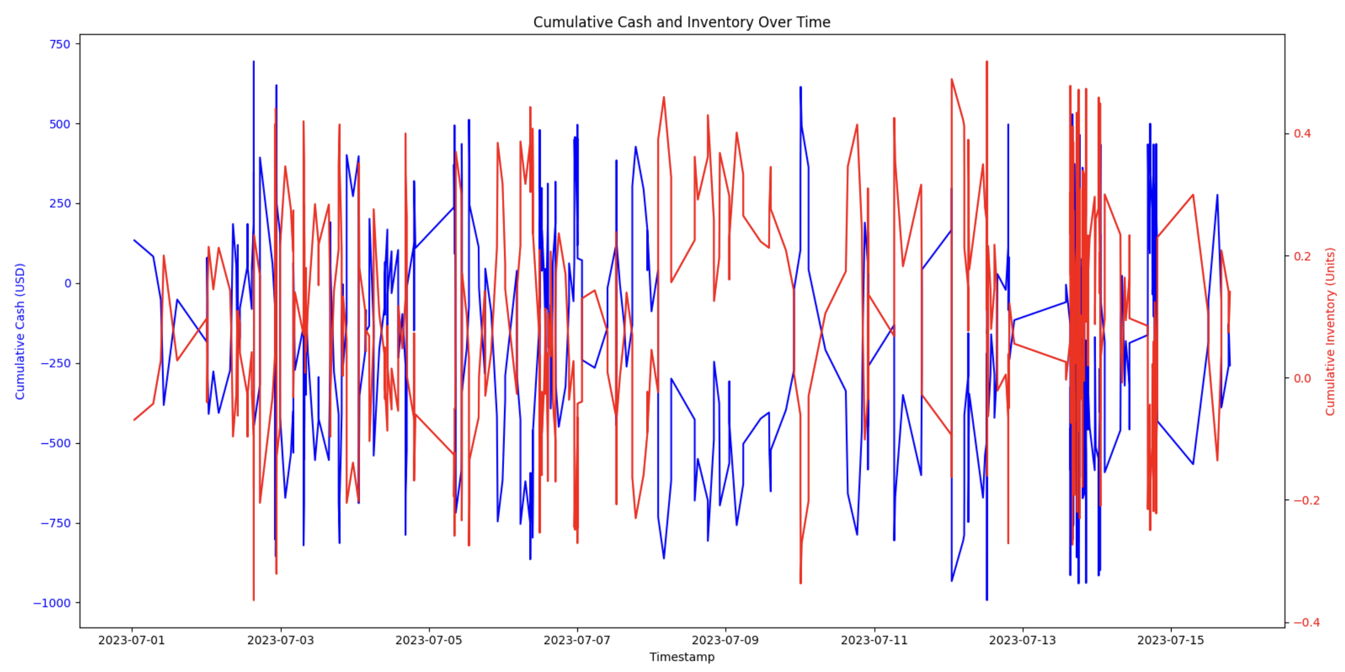
3.1 Visualise Cumulative Cash and Inventory
A time-series plot is used to visualise cumulative cash flow and cumulative inventory:
- Cumulative cash (blue line) - Tracks the net profit or loss in USD over time
- Cumulative inventory (red line) - Measures the total amount of assets held at any given moment
It is easier to see how cash flow is influenced by inventory changes by plotting these metrics together with separate y-axes.
# Visualize cumulative cash and inventory over time
fig, ax1 = plt.subplots(figsize=(16,8))

# Plot cumulative cash on the primary y-axis (left)
ax1.plot(fills_data.index, fills_data['cumulative_cash'], label='Cumulative Cash', color='blue')
ax1.set_xlabel('Timestamp')
ax1.set_ylabel('Cumulative Cash (USD)', color='blue')
ax1.tick_params(axis='y', labelcolor='blue')

# Plot cumulative inventory on a secondary y-axis (right)
ax2 = ax1.twinx()
ax2.plot(fills_data.index, fills_data['cumulative_inventory'], label='Cumulative Inventory', color='red')
ax2.set_ylabel('Cumulative Inventory (Units)', color='red')
ax2.tick_params(axis='y', labelcolor='red')

plt.title("Cumulative Cash and Inventory Over Time")
fig.tight_layout()
plt.show()
Output:
3.2 Find the Correlation Between Cash and Inventory
To evaluate the relationship between cash flow and inventory levels, the correlation coefficient is calculated. A value near -1 indicates an expected inverse relationship in market-making, where buying reduces cash and selling increases it. Deviations from this may signal inefficiencies.
- -1 (Perfect Negative Correlation) – Indicates efficient inventory management, where cash decreases with purchases and increases with sales
- 0 (No Correlation) – Suggests irregular trading behaviour/external influences affecting cash and inventory independently
- 1 (Perfect Positive Correlation) – Uncommon in market-making as it suggests both cash and inventory increase together, potentially indicating inefficient inventory management
# Determine if cash gains/losses are aligned with inventory adjustments
correlation = fills_data['cumulative_cash'].corr(fills_data['cumulative_inventory'])
print("Correlation between Cumulative Cash and Inventory:", correlation)
Output:
Correlation between Cumulative Cash and Inventory: -0.9996847478502905
This near-perfect negative correlation suggests that cash movements are closely tied to inventory adjustments, which aligns with the nature of market-making, where assets are constantly bought and sold while maintaining an inventory balance.
3.3 Measure Inventory Volatility
The standard deviation of cumulative inventory is calculated to quantify inventory volatility. A higher standard deviation implies greater fluctuations in inventory levels, indicating more aggressive trading behavior or market instability. This measure helps in assessing how stable the strategy’s inventory management is over time.
# Calculate the standard deviation of cumulative inventory as a measure of volatility
inventory_volatility = fills_data['cumulative_inventory'].std()
print("Inventory Volatility (Std Dev):", inventory_volatility)
Output:
Inventory Volatility (Std Dev): 0.18185536609357372
A moderate level of volatility (Std Dev ≈ 0.18 ETH) suggests the strategy is generally keeping inventory near its target.
Step 4: Realised and Unrealised Profit and Loss Calculation
This section evaluates the financial performance of the market-making strategy by calculating both realised and unrealised profit and loss (PnL). The analysis employs the average cost method to dynamically track inventory costs and assess trade outcomes over time. This helps gauge the true profitability of the strategy while keeping tabs on open positions.
4.1 Determine Target Inventory
The first step is to infer the target inventory by calculating the median balance held during the trading period. This target acts as a benchmark against which deviations in held inventory are measured. The target inventory serves as a reference point to quantify inventory fluctuations and assess position imbalances.
target_inventory = fills_data['balance'].median()
print("Inferred Target Inventory (median of balance):", target_inventory)
Output:
Inferred Target Inventory (median of balance): 0.5459000000000004
In this example, the median balance indicates a target inventory of approximately 0.546 ETH, suggesting that the strategy aims to maintain its holdings around this level.
4.2 Calculate Realised and Unrealised Profit and Loss
Realised PnL is derived from executed trades by comparing the trade price to the average cost of the inventory:
- Buying (
B) increases inventory and updates the cost basis by adding the purchase price and any associated fees - Selling (
S) realises a profit or loss by comparing the sale price with the current average cost of the held inventory - Cumulative Realised PnL maintains a running total of the profits (or losses) from all completed trades, thus providing a historical perspective on the strategy’s performance
After each sale, the total inventory and cost basis are adjusted to reflect the new position, ensuring that the average cost remains accurate.
Unrealised PnL, on the other hand, represents the potential profit or loss from the current inventory position based on its deviation from the target inventory:
- When excess inventory is held (i.e. above the target), unrealised PnL assumes that the surplus would be sold at the current bid price
- When there is a deficit in inventory (i.e. below the target), it assumes that the shortfall would be purchased at the current ask price
- If there is zero inventory, unrealised PnL is naturally zero since there are no assets to assess
Realised PnL captures the outcome of completed trades, while unrealised PnL estimates the market value of open positions and highlights potential risks if the held inventory deviates significantly from the target.
The following code iterates over each trade in the fills data to:
- Update the cost basis and inventory based on whether the trade was a buy or a sell
- Calculate realised profit or loss on sales
- Adjust the cumulative realised PnL
- Compute the current average cost of the remaining inventory
- Estimate unrealised PnL based on deviations from the target inventory
# Compute realized PnL using an average cost method
# At each fill, update cost basis and inventory
total_inventory = 0.0
total_cost = 0.0
realized_pnl_list = []
avg_cost_list = []
unrealized_pnl_list = []
cumulative_realized_list = []

cumulative_realized = 0.0

for row in fills_data.itertuples():
    if row.side == 'B':
        # If buying, increase inventory and update total cost (including fees)
        total_cost += (row.fill_prc * row.fill_qty) + row.fee_usd
        total_inventory += row.fill_qty
        realized = 0.0
    elif row.side == 'S':
        # If selling, realize PnL using the average cost of the current inventory
        if total_inventory <= 0:
            realized = 0.0
        else:
            avg_cost = total_cost / total_inventory  # Calculate the average cost of held inventory
            qty_sold = min(row.fill_qty, total_inventory)  # Binance doesn't sell more than it has
            cost_of_sale = avg_cost * qty_sold  # Cost basis for the quantity sold
            sale_proceeds = (row.fill_prc * qty_sold) - row.fee_usd  # Cash received from the sale minus fees
            realized = sale_proceeds - cost_of_sale  # Profit or loss on the trade

            # Reduce total inventory and adjust cost basis accordingly
            total_cost -= cost_of_sale
            total_inventory -= qty_sold

    # Update cumulative realized PnL
    cumulative_realized += realized
    realized_pnl_list.append(realized)
    cumulative_realized_list.append(cumulative_realized)

    # Compute the current average cost of the remaining inventory
    current_avg_cost = total_cost / total_inventory if total_inventory > 0 else 0.0
    avg_cost_list.append(current_avg_cost)

    # Estimate unrealized PnL based on the deviation from the target inventory
    if total_inventory == 0:
        unrealized = 0.0
    # If holding excess inventory, assume it would be sold at the current bid price
    elif total_inventory > target_inventory:
        deviation = total_inventory - target_inventory
        unrealized = deviation * (row.bid_prc - current_avg_cost)
    # If holding less than target inventory, assume buying the shortfall at the current ask price
    elif total_inventory < target_inventory:
        deviation = target_inventory - total_inventory
        unrealized = -deviation * (current_avg_cost - row.ask_prc)
    else:
        unrealized = 0.0
    unrealized_pnl_list.append(unrealized)
4.3 Store Computed PnL Metrics
After processing all trades, the computed metrics are appended to the dataset. These metrics include:
- Realised PnL - Profit or loss from executed trades.
- Cumulative Realised PnL - The running total of realised gains or losses.
- Average Cost of Open Inventory - The current cost basis of the remaining holdings.
- Unrealised PnL - The estimated profit or loss from the remaining inventory.
- Total PnL - The sum of realised and unrealised PnL, reflecting the overall profitability of the strategy.
# Append computed metrics to fills_data
fills_data['realized_pnl'] = realized_pnl_list
fills_data['cumulative_realized'] = cumulative_realized_list
fills_data['avg_cost_open'] = avg_cost_list
fills_data['unrealized_pnl'] = unrealized_pnl_list
fills_data['total_pnl'] = fills_data['cumulative_realized'] + fills_data['unrealized_pnl']
4.4 Evaluate Final Performance
The final performance metrics are then displayed.
# Overall performance metrics
print(f"Final Realized PnL: ${fills_data['cumulative_realized'].iloc[-1]:.2f}")
print(f"Final Unrealized PnL: ${fills_data['unrealized_pnl'].iloc[-1]:.2f}")
print(f"Total PnL: ${fills_data['total_pnl'].iloc[-1]:.2f}")
print(f"Total Fees Paid: ${fills_data['fee_usd'].sum():.2f}")
Output:
Final Realized PnL: $20.29
Final Unrealized PnL: $0.06
Total PnL: $20.35
Total Fees Paid: $5.41
Final Realised PnL is $20.29, representing the profit secured from fully executed, closed trades. Final Unrealised PnL is $0.06, indicating that the profit or loss from open positions is negligible. Total PnL is $20.35, the sum of realised and unrealised profit, while Total Fees Paid is $5.41, reflecting the trading costs incurred and deducted from the gross profits.
Overall, the strategy is profitable with controlled inventory levels, as realised profit significantly exceeds both unrealised PnL and fee costs. After accounting for fees, the strategy delivers a modest profit with low exposure to unrealised market risk. The stable target inventory and close alignment between realised profits and inventory adjustments suggest effective inventory management.
Step 5: Profit and Loss Breakdown
This section breaks down the realised profit and loss (PnL) by different trade dimensions to better understand the contributions from various aspects of the strategy.
5.1 Break Down Realised PnL by Trade Side
Realised PnL is aggregated by trade side to reveal the performance of buy and sell transactions. This breakdown helps distinguish the profitability of each side of the market-making operation.
# Realized PnL by trade side
realized_pnl_by_side = fills_data.groupby('side')['realized_pnl'].sum()

print("Realized PnL by Trade Side:")
for side, pnl in realized_pnl_by_side.items():
    trade_type = "Buy" if side == "B" else "Sell"
    print(f" - {trade_type}: ${pnl:.2f}")
Output:
Realized PnL by Trade Side:
 - Buy: $0.00
 - Sell: $20.29
The output indicates that there is no realised profit from buy trades, while sell trades contribute a realised profit of $20.29. This makes sense because profit is only realised through selling.
5.2 Assess Realised PnL by Liquidity Role
Next, the realised PnL is grouped by liquidity role (Maker/Taker) to assess which role contributes more to profitability. This analysis can offer insights into how different execution types affect the overall performance.
# Realized PnL by liquidity role
realized_pnl_by_liquidity = fills_data.groupby('liquidity')['realized_pnl'].sum()

print("Realized PnL by Liquidity Role:")
for role, pnl in realized_pnl_by_liquidity.items():
    print(f" - {role}: ${pnl:.2f}")
Output:
Realized PnL by Liquidity Role:
 - Maker: $16.33
 - Taker: $3.96
Here, the majority of realised profit comes from acting as a Maker (16.33 dollars), while Taker trades contribute a smaller amount (3.96 dollars). This suggests that the strategy is prioritising passive order placement, as maker trades benefit from capturing the bid-ask spread along with lower fees or exchange rebates. Conversely, the lower realised profit from Taker orders indicates that aggressive execution is used sparingly, likely as a risk management measure to quickly adjust inventory when market conditions become unfavourable.
Step 6: Time-Series Analysis of Profit and Loss
This section examines how the strategy’s total PnL evolves over time by analysing its daily fluctuations. Tracking PnL on a time-series basis helps identify trends, volatility, and potential inefficiencies in the market-making approach.
6.1 Visualise Daily Total PnL
A time-series plot of daily total PnL is generated to observe how profitability changes over time. Each day’s PnL is calculated as the difference between the total PnL at the end of consecutive days.
# Daily total PnL time series plot
fills_data['date'] = fills_data.index.date
daily_pnl = fills_data.groupby('date')['total_pnl'].last().diff().fillna(0)

plt.figure(figsize=(12,6))
plt.plot(daily_pnl.index.astype(str), daily_pnl.values, marker='o', linestyle='-')
plt.xlabel('Date')
plt.ylabel('Daily Total PnL (USD)')
plt.title('Daily Total PnL Time Series')
plt.xticks(rotation=45)
plt.tight_layout()
plt.show()
Output:
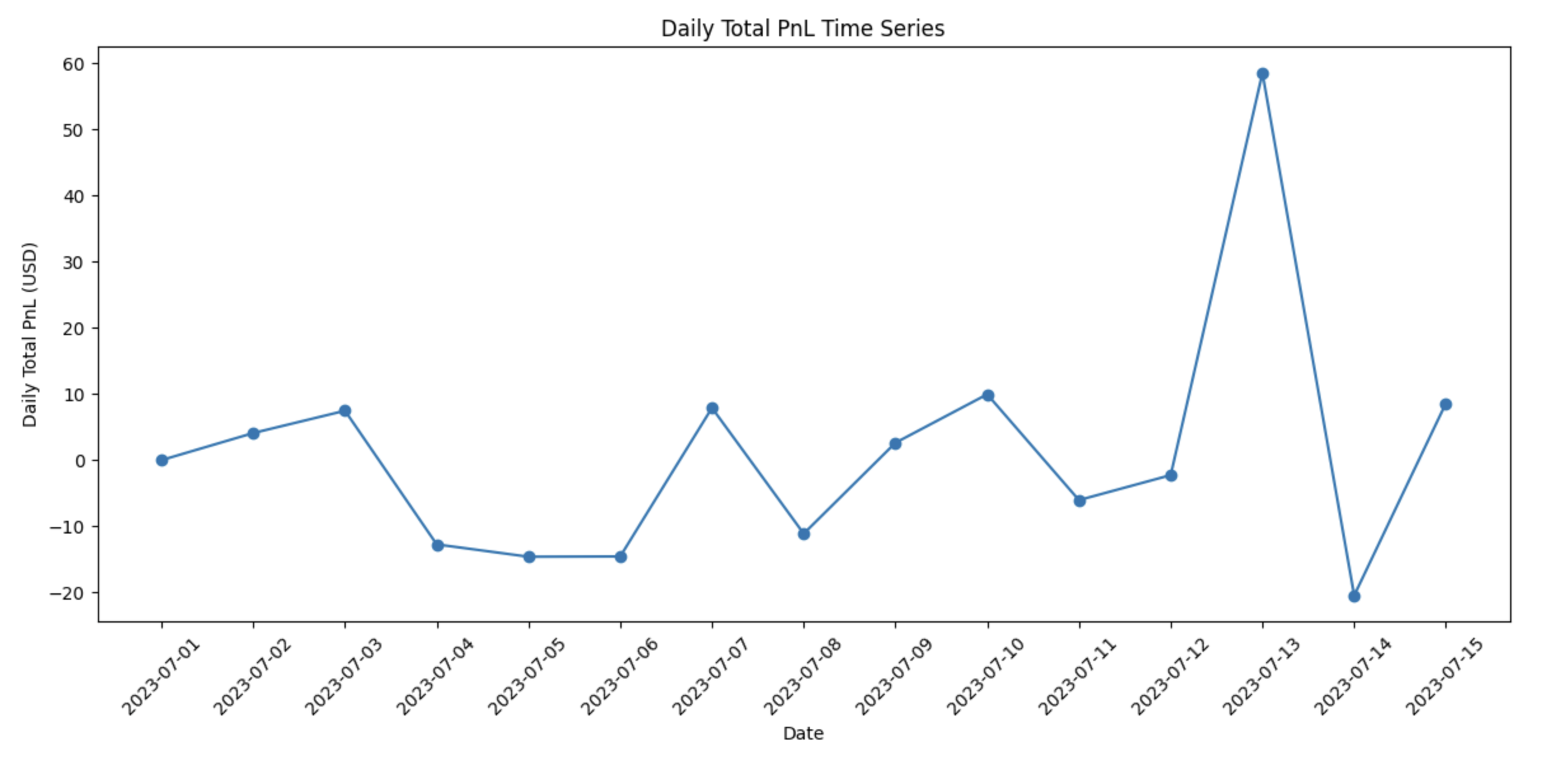
The strategy’s PnL varies from day to day. This indicates sensitivity to market conditions and price movements. Despite this volatility, multiple days show net gains, indicating that the market-making approach remains profitable over the long term. However, significant drawdowns may suggest inefficiencies in inventory management or increased reliance on taker orders at unfavourable prices.
Step 7: Price Behaviour Analysis After Fills
This section examines the immediate market reaction following each fill by analysing the 1-minute return. Focusing on this short interval isolates the direct effect of a trade, reducing interference from later market fluctuations, and provides a robust measure of execution quality and potential slippage. Other time windows (e.g. 5 or 15 minutes) might blend these immediate effects with broader market movements or news events that are less directly tied to the specific trade.
7.1 Merge Future Market Data
For each fill, the timestamp is advanced by one minute to capture the corresponding market prices (bid and ask) at that future moment. This technique ensures that the subsequent market reaction is accurately recorded, reflecting any rapid price adjustments post-execution.
# Convert both indexes to nanosecond precision
market_data.index = market_data.index.astype('datetime64[ns]')
fills_data.index = fills_data.index.astype('datetime64[ns]')

# Create a new column for timestamp shifted by one minute.
fills_data['timestamp_plus_1min'] = fills_data.index + pd.Timedelta(minutes=1)

# Merge forward bid/ask prices from market_data
fills_data = pd.merge_asof(
    fills_data,
    market_data[['bid_prc', 'ask_prc']].rename(columns={'bid_prc': 'bid_1min', 'ask_prc': 'ask_1min'}),
    left_on='timestamp_plus_1min',
    right_index=True,
    direction='forward'
)
7.2 Calculate 1-Minute Returns by Trade Side
The 1-minute return is calculated separately for buy and sell fills. For buy fills, the return is derived from the difference between the future ask price and the fill price; for sell fills, it is based on the difference between the fill price and the future bid price. This calculation quantifies the immediate profitability of each trade and identifies any short-term execution advantages.
# Compute 1-minute return based on trade side
fills_data['return_1min'] = np.where(
    fills_data['side'] == 'B',
    (fills_data['ask_1min'] - fills_data['fill_prc']) / fills_data['fill_prc'],
    (fills_data['fill_prc'] - fills_data['bid_1min']) / fills_data['fill_prc']
)
7.3 Visualise 1-Minute Return Distribution
A histogram is used to depict the distribution of 1-minute returns for both trade sides. This visualisation highlights the frequency and range of positive and negative returns. For example, a slightly higher average return for buy fills may indicate a marginally more favourable market response when entering long positions. Such analysis aids in assessing execution performance and refining trade timing.
# Plot the distribution of 1-minute returns by trade side
plt.figure(figsize=(10,6))
sns.histplot(data=fills_data, x='return_1min', hue='side', kde=True, bins=30)
plt.title("Distribution of 1-Minute Returns After Fills")
plt.xlabel("1-Minute Return")
plt.ylabel("Frequency")
plt.show()
Output:
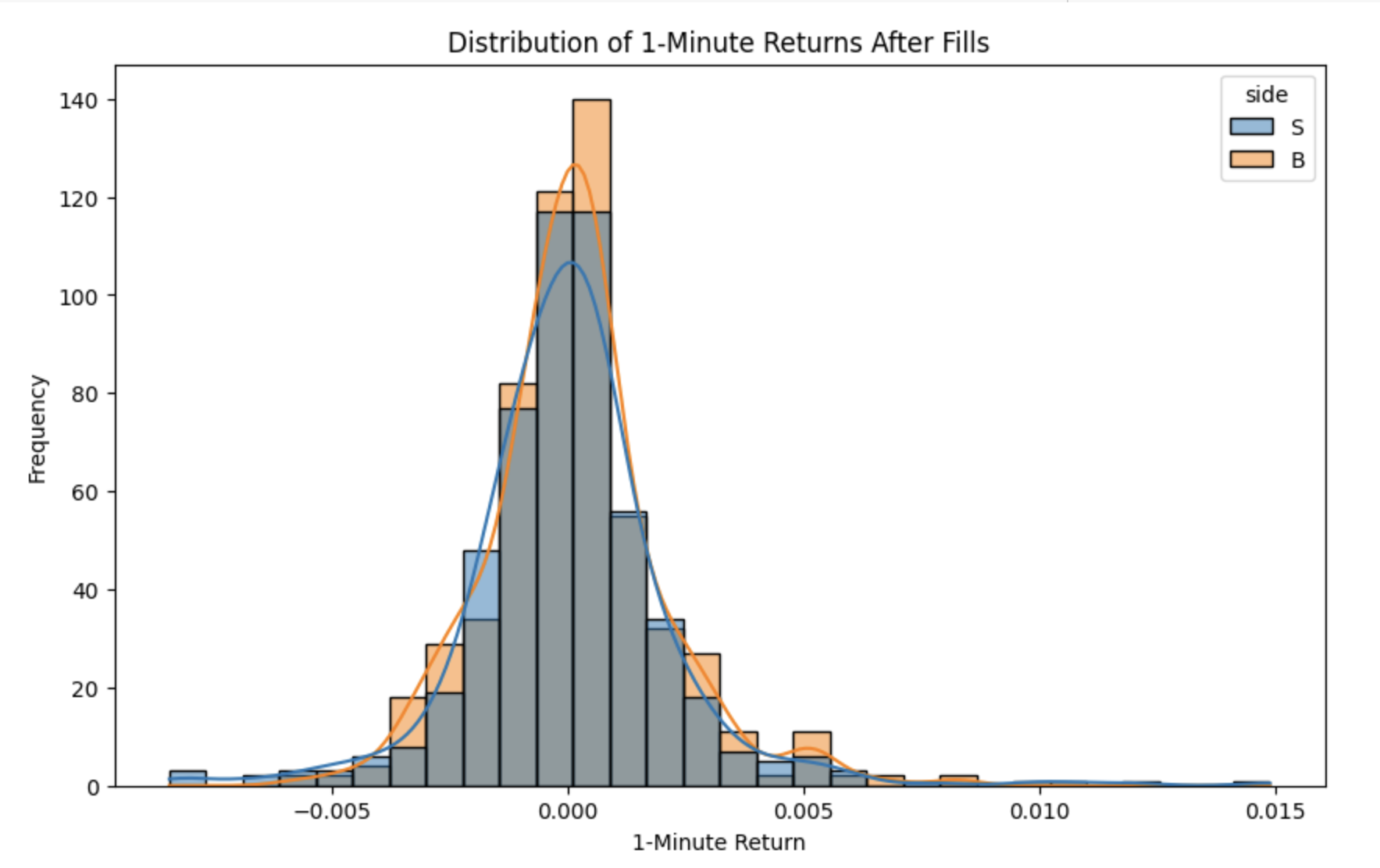
The 1-minute returns for both buy (B) and sell (S) fills cluster around zero. It means prices typically do not move dramatically in the minute after a fill. The bell-shaped curves imply that small price movements (positive/negative) are more common than large swings, indicating relatively efficient market conditions. This pattern implies that market participants quickly absorb new orders without causing significant short-term dislocation, which can be advantageous for strategies aiming to capture small, consistent profits through frequent trades.
7.4 Examine 1-Minute Returns by Trade Side
Presenting average returns separately for each side clarifies differences in short-term performance between buy and sell orders. This practice reveals whether market conditions around execution systematically favour one action over the other. A comparison of mean 1-minute returns highlights which side tends to achieve a slightly better outcome.
# Summary statistics for 1-minute returns by trade side
print("Average 1-Minute Return by Side:")
summary_stats = fills_data.groupby('side')['return_1min'].mean().reset_index()
display(summary_stats)
Output:
Average 1-Minute Return by Side:
  side    return_1min
0    B       0.000122
1    S       0.000028
Buy fills show a mean return of 0.000122, while sell fills stand at 0.000028, indicating a marginal edge for buying in the immediate timeframe. This result may reflect a mild upward bias or faster price recovery after purchase. A higher average return for buy trades could justify stronger inventory replenishment if the market frequently rebounds soon after entry. It may also lead to a review of quoting widths on the sell side to reduce potential slippage or secure gains more efficiently.
7.5 Assess Performance Metrics
A broader set of measures, such as win rate, average gain, and average loss, demonstrates how often trades turn a profit within the one-minute window and the typical magnitude of those gains or losses. The win rate captures the proportion of trades that realise a positive return at the one-minute mark, while average gain and loss detail how much is typically won or lost during this brief period.
# Performance Metrics
win_rate = (fills_data['return_1min'] > 0).mean() * 100
avg_gain = fills_data[fills_data['return_1min'] > 0]['return_1min'].mean()
avg_loss = fills_data[fills_data['return_1min'] < 0]['return_1min'].mean()

print(f"Win Rate: {win_rate:.2f}%")
print(f"Average Gain: {avg_gain:.6f}")
print(f"Average Loss: {avg_loss:.6f}")
Output:
Win Rate: 51.29%
Average Gain: 0.001414
Average Loss: -0.001360
A win rate above 50% means the price moves on average in the strategy’s favor just over half the time within the first minute after a fill. It suggests that small yet consistent gains may accumulate over multiple trades. Even a modest advantage in these figures can have a material influence on long-term returns. This highlights the importance of careful execution timing and continuous monitoring of fills in a market-making strategy.
Step 8: Trade Execution and Liquidity Metrics
This section evaluates the strategy’s trade execution and liquidity by summarising key metrics along two dimensions: trade side (Buy/Sell) and liquidity role (Maker/Taker). These summaries reveal how different order types contribute to overall performance and assist in assessing execution efficiency.
8.1 Break Down Trade Activity
Trades are classified as either buy or sell, and for each category, metrics such as the total number of trades, average fill quantity, total traded volume, and average fill price are computed. This breakdown illustrates the balance between buying and selling activities, which is crucial for maintaining effective inventory management.
# Create a summary of trade statistics based on the 'side' column (Buy/Sell)
trade_summary = fills_data.groupby('side').agg(
    trades=('order_id', 'count'),
    avg_fill_qty=('fill_qty', 'mean'),
    total_volume=('fill_qty', 'sum'),
    avg_fill_price=('fill_prc', 'mean')
).reset_index()

print("Trade Summary by Side:")
display(trade_summary)
Output:
Trade Summary by Side:
  side    trades    avg_fill_qty    total_volume    avg_fill_price
0    B       580        0.067994         39.4367       1934.553155
1    S       543        0.072369         39.2963       1934.720424
The near parity between 580 buy trades (averaging ~0.068 ETH each, totalling ~39.44 ETH) and 543 sell trades (averaging ~0.072 ETH each, totalling ~39.30 ETH) suggests tight execution and effective inventory management.
8.2 Assess Liquidity Contribution
Trades are also grouped by liquidity role to evaluate the impact of different order types on profitability. Liquidity refers to how easily an asset can be bought or sold in the market without significantly affecting its price. Maker orders provide liquidity and often earn lower fees or exchange rebates, while taker orders are executed immediately against existing orders and typically incur higher costs. These roles also reflect different execution strategies: maker orders are considered passive since they add liquidity to the market, whereas taker orders are viewed as aggressive because they remove liquidity.
# Create a summary of liquidity statistics grouping by the 'liquidity' column (Maker/Taker)
liquidity_summary = fills_data.groupby('liquidity').agg(
    trades=('order_id', 'count'),
    avg_fill_qty=('fill_qty', 'mean'),
    total_volume=('fill_qty', 'sum'),
    avg_fill_price=('fill_prc', 'mean'),
    total_realized_pnl=('realized_pnl', 'sum')
).reset_index()

print("\nLiquidity Summary:")
display(liquidity_summary)
Output:
Liquidity Summary:
  liquidity    trades    avg_fill_qty    total_volume    avg_fill_price    total_realized_pnl
0     Maker      1038        0.063687         66.1076       1935.721599             16.328486
1     Taker        85        0.148534         12.6254       1921.352941              3.960174
The liquidity summary reveals that maker orders dominate, contributing the majority of the realised profit (16.33 dollars), while taker orders, although less frequent and larger in size, contribute a smaller profit (3.96 dollars). This indicates that the strategy predominantly employs passive order placement to capture the bid-ask spread and benefit from lower fees or exchange rebates, with taker orders used sparingly for quick inventory adjustments when market conditions deteriorate.
Closing Remarks
The realised PnL comes mainly from passive fills, which is consistent with a spread-capture style strategy rather than directional trading. Inventory is kept close to its target, which limits exposure to price drift, but taker usage tends to cluster when the book moves against the strategy, suggesting rebalancing is mostly reactive.
The dataset only covers a short window, so it does not show how the behaviour changes in stressed or low-liquidity conditions. A natural next step would be to measure adverse selection more directly by looking at midprice moves after execution and to test whether the same inventory behaviour holds when spreads compress or volatility increases.
Across this period, the strategy is profitable, but the edge comes from microstructure (earning the spread) rather than forecasting price direction.